




This article was inspired by the discussion thread under an article I published early in the off-season.
That article showed that Mike Sainristil was among the most productive CBs at intercepting the football in 2025, but was also well below average at rate of yardage allowed in coverage, and close to the worst in the league at giving up scores. If memory serves me correctly, it was Hogs Haven regular shally who posed the question that gave this article its title.
In fact, that question was really
just the excuse I needed to take on a topic that I had wanted to write about since the Commanders parted ways with WR/PR Dax Milne after the 2022 season.
Those readers who remember Dax may recall that he was right on the league average in return yardage, but had very good hands and never fumbled. That led to some debate among the regular commenters about whether it was better to have a plodding punt returner who never fumbles or a big play threat who occasionally fumbles. To shed some light on that topic I embarked on what turned out to be my largest ever number crunching project for Hogs Haven. When I was about half-way through, the Commanders released Dax, making it no longer topical. So I shelved it and moved on to other topics.
Conceptually, the Dax Milne debate boiled down to the same fundamental question which was posed about Mike Sainristil: How can we equate the value of two entirely different types of play outcomes? It turns out that big punt returns vs. fumbles can be answered in exactly the same way as interceptions vs big gains and TDs allowed in coverage. Except in the latter case, the numbers are readily available without a lot of extra work.
The key to solving this puzzle is Expected Points Added, more commonly abbreviated as EPA. EPA has gained new life recently as one of the predictive measures used in sports betting and fantasy football. It was developed by statisticians Bob Carroll, John Thorn and Pete Palmer in their seminal work The Hidden Game of Football, which played a big part in ushering in the modern era of football analytics.
EPA provides a common currency to equate the value of any two plays in football. It is based on a statistical model of the football field derived from over a decade of play-by-play data from every game by every team in the league. The model makes it possible to calculate the Expected Points at the start and end of any play. The Expected Points are the average number of points scored on a drive by a team starting at a given down and distance from a given field position. EPA is simply the Expected Points at the end of the play, minus the Expected Points at the start. I’ll provide an example later, when we start delving into Mike’s plays in coverage.
EPA quantifies a play’s impact on the offense’s expectations for scoring on the current drive. The key to its versatility is that it doesn’t matter what happened on the play. Consequently, we can use it to compare very different types of plays, such as a fumble and a punt return for a TD, or an interception and a TD reception allowed in coverage, as just two examples.
There are some limitations. Most notably, to use EPA to measure individual performance, we have to be able to attribute the entire play outcome to a single player. While no play is ever entirely an individual effort, for the types of plays we will be looking at here – interceptions and receptions allowed in coverage – I think it is a reasonable approximation to attribute outcomes to the primary defender in coverage (noting here that Mike had help from Johnny Newton on his third-biggest interception of the season). To avoid getting lost in the weeds, that’s all I’ll say about the technicalities now. Readers are invited to take up the finer points in the comments if they like.
Running with the common currency concept, I used an accounting approach in which I asked whether the EPA credits Mike banked by making more interceptions than expected was enough to pay off the debt he accumulated by allowing more than expected negative plays in coverage.

Opening Balances
For this accounting exercise, I used play-by-play and EPA data from the Pro Football Reference (PFR) Stathead database. It is worth noting that PFR’s advanced coverage stats were kinder to Mike’s 2025 performance than those from Pro Football Focus (PFF). Since PFF doesn’t provide access to the play-by-play data, which was needed for this analysis, I stuck with the tool which would do the job.
According to PFR, Mike allowed 733 yds and 9 TDs in coverage in the 2025 regular season. Those figures ranked 7th and 2nd highest, respectively, among NFL CBs in the regular season.
However, it might be a little unfair to compare Mike to other CBs based on cumulative totals, because he also played the 8th most coverage snaps among NFL CBs, and therefore faced more opportunities than most to accumulate negative plays.
To make sure we are ranking Mike fairly against the rest of the league, we need to adjust for differences in playing time by converting the totals to productivity rates.
Yardage Allowed. Using PFR’s figures, Mike allowed 1.21 Yards/Coverage Snaps, which was the 79th highest (24th worst) among 103 CBs (min 233 coverage snaps). Correcting for playing time makes him look better than the cumulative total. But he was still well below league average.
Touchdowns Allowed. The biggest issue with Mike’s coverage was allowing touchdowns. To make fair comparisons I converted the raw TD totals to TD Rates, expressed as the percentage of coverage snaps with a TD allowed. Mike gave up TDs on 1.4% of coverage snaps, which was the 4th highest TD Rate among the 103 most active CBs. He got less benefit from adjusting the TD totals for playing time than he did with yardage allowed.
Now let’s calculate his balance owing. It would be unfair to expect a CB to allow 0 yardage or TDs in coverage. The league rules are tilted to favor the offense in the passing game. Even the best starting CB is going to give up some yardage in coverage.
A more reasonable expectation for any starting player is the league average for their position. The league average Rate of Yardage Allowed for CBs using PFR’s data was 1.04 Y/Cov Snap. The average CB, playing the same amount of coverage snaps as Mike (607 snaps), would therefore be expected to give up 631 yards. Mike was just 100 yards, or 15.8% above expectation, after correcting for rounding errors.
If yardage were the only issue, then Mike’s debt to the team would not be too hard to pay off. The bigger issue was scores allowed. Mike’s 1.4% TD Rate in coverage was more than twice the league average of 0.625%. The average CB playing 607 coverage snaps would be expected to allow 3.8 TDs, which rounds to 4. Mike allowed 9 TDs, which placed him 5 TDs (125%) over expectation. That is a harder debt to pay off.
Interceptions. On the positive side of the ledger, Mike was one of the best CBs in the league at intercepting the football. His 4 interception total placed him in a 6-way tie for 2nd most among CBs in the regular season. Only Jaycee Horn and Nashon Wright were ahead of him at 5 INTs in regulation.
Correcting for numbers of opportunities, by calculating Interception Rate (% of targets intercepted), drops him to 11th best, or 89th percentile of the 103 most active CBs. Mike intercepted an impressive 4.49% of his targets, nearly three times the league average of 1.52%. The average CB would be expected to intercept 1.3 of the 89 targets Mike faced, which rounds down to 1.
That gives Mike a positive balance of 3 interceptions above expectation to pay toward the debts he accumulated in the yardage- and TD-over-expectation columns. Will it be enough?

Paying Off the Debt
To answer that question, let’s tally up the EPA values from Mike’s biggest three interceptions to get his credit balance, then start deducting his negative plays in coverage to see how far that takes him. He needs to pay off 100 coverage yards and 5 TDs over expectation.
Before we get started, I need to point out that EPA is counted from the perspective of the offense. Since Mike plays on defense, plays with positive EPA are good for the Commanders’ opponent. Mike’s interceptions have negative EPA, as do any other positive plays he made on defense. Just remember, negative is good and positive is bad. Sorry if that’s confusing.
EPA Credit Balance
Mike’s biggest three interceptions in 2025 are shown in the following table, along with the EPA values for the plays in which they occurred. The fourth was a pick on 3rd and 4 in the third quarter against the Seahawks with an EPA of -3.22. To give Mike the maximum possible spending power (a.k.a. erring in his favor) let’s treat that one as the one interception he was expected to make.

An Aside – EPA Illustrated: To illustrate how EPA works, let’s take a look at the big interception against the Giants. The Giants started the play at 2nd and 4 on the Washington 35 yard line, with hopes of scoring once more to narrow the Commanders’ lead before the half. Their Expected Points at the start of the play were 3.12. Teams in that position on second down have a good chance of scoring a field goal on their drive, and have a fair chance of scoring even more.
Mike picked off Jaxson Dart’s pass at the Washington 21 and returned it 55 yards to the Giants’ 24 yard line with 10 seconds remaining in the half. The Commanders start their next drive with 3.97 Expected Points. But because we are counting EPA for the play from the Giants’ perspective, that becomes -3.97 Expected Points. The EPA for the play is the Giants’ Expected Points at the end of the play minus their Expected Points at the start: EPA = -3.97 – 3.12 = 7.09.
Mike’s interception flipped the script, taking the Commanders from a game situation where the most likely outcome was a field goal for the other team to one where they were expected to score a field goal and change. Two plays later, Jake Moody kicked a 42-yard field goal to extend the Commanders’ lead at the half, in line with the expection.
Paying Down the Debt
Back to the main story, Mike banked -16.44 EPA with his interceptions. Let’s see how far that goes toward paying off the debt from his negative plays in coverage.
I started by ranking the negative plays in descending order of EPA. The top four were TD receptions. Mike didn’t have enough credit banked to pay for the fourth one, so I put it back. That left him with a remaining credit balance of -1.94.
Scrolling down the list to the next two negative plays he could afford brought me to two receptions he allowed for similar yardage on third and long. A 3rd and 9 completion for 12 yards by the Vikings for 1.96 EPA was 0.02 EPA above his credit balance, while a 13-yard completion by the Dolphins on 3rd and 7 was just under at 1.90. Two hundredths of an Expected Point is nothing in the scheme of things, so I let him have the slightly more valuable play. Here are the four negative plays he paid off with his interceptions over expectation:

Remaining Balances
By cashing in the credits he banked with 3 interceptions over expectation, Mike was able to pay off the debts he accumulated from the three biggest TD receptions he allowed, plus a 12-yard receception for a conversion on third down. The four negative plays he paid for totalled 114 receiving yards. Therefore, his three interceptions over expectation completely cleared his debt for allowing more yardage than expected, with 14 yards to spare.
With that debt cleared, all we have to worry about are the two remaining unpaid TDs over expectation. Assigning EPA values to those plays is a little challenging, because it’s not clear which of the 6 remaining TD receptions to count.
If we want to make it as hard as possible for Mike, we could make it the two TD receptions with the next highest EPA values. Those were a 9-yard TD reception by the Lions’ Amon-Ra St Brown and an 18-yard TD catch by the Vikings’ Josh Oliver, which totalled 5.93 EPA.
A more reasonable approach might be to assign them the average value of the remaining 6 TDs, which comes to 1.89 EPA. Multiplying by 2 gives a more manageable figure of 3.78 EPA.
Let’s use those two figures to see how much more Mike would have needed to do to balance the books for the 2025 season.
How Many Interceptions Did Mike Sainristil Owe the Commanders?
The final step is to calculate the number of additional interceptions Mike would have needed to make to pay off his remaining debt for the two remaining TD receptions over expectation. In the previous section I calculated that debt at somewhere between 3.78 and 5.93 EPA.
For this step, we need to place a value on interceptions that Mike didn’t make. The most reasonable approach is to use the average value of the four interceptions he did make: -4.91 EPA.
Using the low estimate (3.78 EPA) Mike’s remaining debt for allowing too many TDs in coverage would have been paid off completely by one additional interception, with excess value to spare. Paying off the higher estimated debt (5.93 EPA) would require 1.2 additional interceptions. Since interceptions are binary, he would need to make up the difference by another play in coverage, such as a pass breakup on third down or another defensive stop.
So the final answer is, Mike fell short of making up for the excess yardage and TDs he allowed in coverage by somewhere between one interception or one interception plus one more reasonably big play.

Summary and Conclusion
In his second NFL season, Mike Sainristil was one of the best CBs in the NFL at making interceptions and among the worst at giving up big plays in coverage. That raised the question, how may interceptions would he have needed to have made to make up for the all the yardage and TDs he gave up in coverage?
Using Expected Points Added (EPA) to establish equivalent value between interceptions and big negative plays, I estimated that he would have needed to make one more interception and possibly another big play or two to clear his debt to the team and bring his value in coverage back to expectations of average play for his position.
There are two ways that we can look at that.
Looking on the bright side, Mike was really only one or two plays away from performing at an average starting level when both positive and negative plays in coverage are taken into account. That doesn’t just go for making interceptions. If not for four big negative plays, his overall performance in coverage would have reached league average. His numbers, reviewed in this article, provide a good illustration of how fine the balance is between above-average and below-average performance at CB. It is not hard to imagine that better communication and better play from others in the secondary would have been enough to flip the balance sheet for him.
On the other hand, Mike made the second-most interceptions at his position in the regular season. In order to wipe the slate clean, to bring his overall performance back to average starting level, he would have needed to have at least tied for the most interceptions by a CB. It is challenging for a CB to earn his living from interceptions alone in the long term. In order to stick as a starter, he will need to get better at containing big gains in coverage than he was in his first two seasons with the Commanders.
To conclude on a positive note, there are big changes to the Commanders defense under way this off-season. When Sainristil was drafted, there were high expectations that he could be a very good nickel corner. In his first two NFL seasons, he has played predominantly on the outside. Entering his third NFL season, it would not be unreasonable to hope that better utilization and scheming might accentuate his strengths, while mitigating his weaknesses in coverage, to allow him to play to his potential.