


The 'K' Is More Art Than Science
The first step in k-means is choosing 'k,' the number of clusters you want to find. In tutorials, this number is usually given to you. Your dataset has three types of flowers? Use k=3. Simple. The first major surprise for practitioners is that in the real
world, you almost never know the right 'k' in advance. Is your company’s user base made of three segments, or seven, or twenty-one? You have to decide. This isn't a minor detail; an incorrect 'k' can render your entire analysis useless, leading to flawed marketing campaigns or nonsensical product categories. While methods like the 'elbow method' or 'silhouette score' exist to help guide this choice, they are heuristics, not magic wands. They provide clues, but often the final decision rests on a combination of these metrics, domain expertise, and the ultimate business goal—a messy, subjective process that classroom exercises rarely prepare you for.
Your Starting Point Can Change Your Destination
The k-means algorithm begins by randomly placing 'k' initial centroids in your data space, then refining them. The word “randomly” should be a warning sign. Depending on where those first points land, you can get wildly different final clusters from the exact same dataset. It’s like dropping parachutists into a mountain range at night; where they land first dramatically affects the base camps they end up establishing. A poor initial placement can lead the algorithm to converge on a 'local optimum'—a decent, but not the best, solution. This means you could run the same analysis twice and get two different answers. In practice, data scientists mitigate this by running the algorithm multiple times with different random starts (a parameter often called 'n_init' in libraries like scikit-learn) and picking the best result. The surprise isn't that this happens, but how often it's overlooked by newcomers who assume one run is enough.
It Assumes Everything Is a Sphere
Here’s the algorithm’s biggest hidden assumption: k-means is designed to find nice, neat, spherical clusters of similar sizes. It defines clusters based on distance to a central point, which naturally creates sphere-like shapes. If your data contains groups that are elongated, intertwined, or have different densities, k-means will struggle and likely fail. Imagine trying to identify a winding river and a small, dense village on a map using only cookie cutters. You’ll carve up the river into arbitrary circular chunks and might capture the village okay, but you’ll completely misunderstand the true shape of the landscape. For many real-world problems, from identifying fraudulent transaction patterns to understanding complex social networks, the underlying groups are not simple blobs. This geometric limitation is a fundamental surprise that forces practitioners to learn other, more flexible clustering algorithms like DBSCAN or spectral clustering.
Scale Matters More Than You Think
Because k-means is based on Euclidean distance, it is highly sensitive to the scale of your features. Let’s say you’re clustering customers using two features: their age (ranging from 20 to 70) and their annual income (ranging from $30,000 to $500,000). The income values are orders of magnitude larger than the age values. When the algorithm calculates distances, the income feature will completely dominate the age feature. The algorithm will essentially ignore age, even if it’s a critically important piece of information for segmentation. The surprise for new practitioners is that failing to 'normalize' or 'standardize' your data before running k-means isn't an optional fine-tuning step; it’s a mandatory prerequisite for a meaningful result. It's the equivalent of comparing measurements in inches and miles without converting them first—the comparison becomes nonsensical.