








The Kernel Trick Feels Like Magic
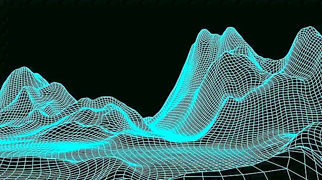
The first major surprise is the 'kernel trick'. In class, you learn that SVMs draw a line (or hyperplane) to separate data. But what if the data isn't linearly separable, like a circle of one class inside another? The kernel trick elegantly solves this.
It's a method that allows the SVM to find a complex, non-linear decision boundary without explicitly doing heavy math. Instead of actually transforming your data into a much higher dimension to make it separable, a kernel function calculates the relationships between points as if they were in that higher space. For a beginner, this feels like a black box. You swap a 'linear' kernel for a 'Radial Basis Function' (RBF) kernel, and suddenly your model draws a perfect circle around the data it couldn't handle before. The surprise is realizing you're getting the power of high-dimensional transformations without the massive computational cost.
Great on Small Data, Sluggish on Big Data
Here's a paradox that trips up many: SVMs are fantastic in high-dimensional spaces (lots of features) but can be surprisingly inefficient with large numbers of samples. You might assume a powerful algorithm scales up easily, but SVM training complexity can increase significantly with the size of the dataset. This is because the classic method involves calculations between pairs of data points. For a huge dataset, this becomes computationally expensive and memory-intensive. Conversely, SVMs excel on small-to-medium datasets, even when the number of features is larger than the number of samples, a scenario common in fields like genomics or medical diagnostics. This is because the decision boundary is defined only by the most critical points, known as support vectors. For newcomers used to algorithms that always want more data, the SVM’s preference for smaller, feature-rich datasets is a genuine surprise.
Performance Lives and Dies by Tuning
A new practitioner might run an SVM with default settings and get mediocre results, then incorrectly conclude the algorithm is weak. The reality is that SVMs are incredibly sensitive to their hyperparameters, particularly 'C' and 'gamma'. These aren't just minor adjustments; they fundamentally change the model's behavior. The 'C' parameter controls the trade-off between having a smooth, wide margin and correctly classifying all training points. A low C allows for a wider margin and some misclassifications (more general), while a high C insists on classifying everything correctly, risking overfitting to the training data. The 'gamma' parameter defines how much influence a single training example has. A small gamma means a point has a far reach, leading to a smoother boundary, while a large gamma means only close-by points have influence, creating a more complex, wiggly boundary. Without carefully tuning these, an SVM can either be too simple or chaotically complex, making hyperparameter optimization an essential, not optional, step.
They Aren't Just for Classification
Most introductory courses frame SVMs purely as a classification tool for sorting data into distinct categories like 'spam' or 'not spam'. It's a surprise for many to learn that the underlying principle can be adapted for regression tasks—predicting continuous values. This variant, known as Support Vector Regression (SVR), flips the objective. Instead of maximizing the margin that separates two classes, SVR tries to fit as many data points as possible within the margin (the 'street'), while limiting margin violations. This makes it a robust tool for regression, especially when dealing with outliers. While not always the go-to for regression problems, its existence demonstrates that the core concepts of maximizing margins and using support vectors are more flexible than they first appear, adding another layer to the SVM toolkit that often surprises practitioners who only know it for its classification prowess.